Shallow neural network exercise

Let’s see if I can write a single hidden layer NN that would be able to say if an image of a floor plan shows a one-room apartment or not.

First, load libraries.

import pandas as pd
import numpy as np
import sklearn
import cv2
import random
import matplotlib.pyplot as plt
import time

Read in the data:

df = pd.read_csv("../../static/data/all_flats_clustered.csv")

Data processing

To make things simple, I’m going to only work with one apartment per shape cluster.

df.drop_duplicates("cluster", keep = "first", inplace = True)

I also only want to keep one- and four-room apartments.

df = df[(df.room_number == 1) | (df.room_number == 4)]

Let’s read in the floor plan images. These are saved locally on my computer, soz… ¯\_(ツ)_/¯

I’ll create an empty array and then append each image in a loop. cv2.imread(x, 0) reads the files in greyscale. I want to normalise the values so that they don’t range between 0 and 255 but 0-1. I also want to get rid of the greyscale by forcing non-white pixels to be black. That is what ... == 1 does and astype(int) casts the resulting boolean as integer.

n = 1000
dims = 112

all_data = []
for i in range(0, df.shape[0]):
    img = cv2.imread("../../../similarity/0" + str(df.room_number.iloc[i]) + "_room/" + str(df.room_number.iloc[i]) + "room_" + df.bfa.iloc[i] + ".png", 0)
    img = cv2.resize(img, (dims, dims))
    all_data.append(((img / 255) == 1).astype(int))

# convert to NumPy array so that it has .shape
all_data = np.array(all_data)

Let’s see if that worked:

plt.imshow(all_data[0], cmap = "gray")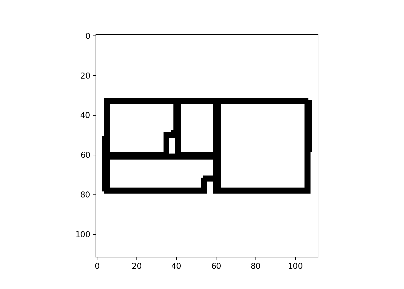

Now, let’s flatten the images, reshaping each to a 1D array.

all_data = all_data.reshape(all_data.shape[0], -1)

df = df["room_number"].values.reshape(df.shape[0], 1) # only keep relevant columns
df = (df == 1).astype(int)

As a final step in data wrangling, I’m creating a 30-70 split of the data into train and test sets.

train_ind = np.random.choice(range(0, df.shape[0]), n, replace=False)
mask = np.zeros(df.shape[0], dtype=bool)
mask[train_ind] = True
X_train = all_data[mask]
Y_train = df[mask]
X_test = all_data[~mask]
Y_test = df[~mask]

Model design

Structure of the neural network. Stolen from Coursera.

Forward propagation

Note

I’m following a linear regression convention below as that’s the one I’m most familiar with. In ML literature, you may find the same equation expressed as \(\mathbf{Z}^{[1]} = \mathbf{W}^{[1]\textsf{T}}\mathbf{X} + b\). This is really the same thing and the difference is only due to the fact that the \(\mathbf{Z}^{[1]}\) and \(\mathbf{W}^{[1]}\) matrices here are transposed with respect to those in ML literature.

\[\mathbf{Z}^{[1]} = \mathbf{X}\mathbf{W}^{[1]} + b^{[1]},\]

where

\[ \mathbf{X} = \begin{bmatrix} x_{11} & \dotsb & x_{1n}\\ x_{21} & \dotsb & x_{2n}\\ \vdots & \ddots & \vdots\\ x_{m1} & \dotsb & x_{mn} \end{bmatrix}, \]

is the \(m\times n\) matrix of \(n\) features for \(m\) training examples (observations).

\[ \mathbf{W}^{[1]} = \begin{bmatrix} w_{11} & w_{12} & w_{13} & w_{14}\\ w_{21} & w_{22} & w_{23} & w_{24}\\ \vdots & \vdots & \vdots & \vdots\\ w_{n1} & w_{n2} & w_{n3} & w_{n4} \end{bmatrix}, \]

is a \(n\times 4\) matrix of weights, with each column representing the weights for one of the four nodes of the hidden layer. Rows contain the regression weights for all of the \(n\) features.

\[ b^{[1]} = \begin{bmatrix} b_1 \\ b_2 \\ b_3 \\ b_4 \end{bmatrix} \]

is a column vector of biases/intercepts.

The resulting matrix \(\mathbf{Z}^{[1]}\) is a \(m\times 4\) matrix of outcomes of this linear regression with one column per node of the hidden layer.

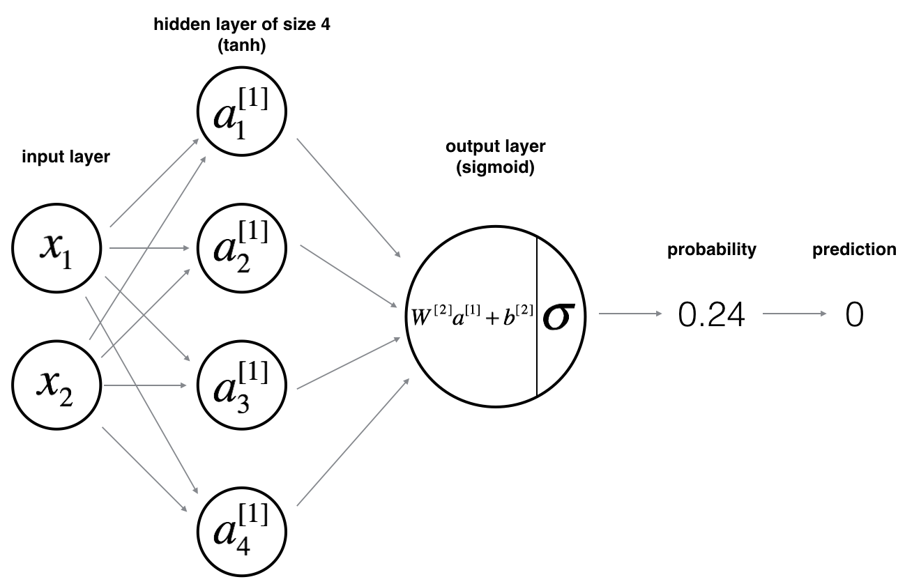
\[ \begin{aligned} \mathbf{A}^{[1]} &= \tanh(\mathbf{Z}^{[1]}) \\ Z^{[2]} &= \mathbf{A}^{[1]}W^{[2]} + b^{[2]} \\ \hat{Y} &= Z^{[2]} = \sigma(Z^{[2]}) \\ y^{(i)}_{pred} &= \begin{cases} 1 & \text{if }\hat{y}^{(i)} > 0.5 \\ 0 & \text{otherwise} \end{cases} \end{aligned} \]

In the above, \(\hat{Y}\) is a column vector of \(m\) predicted probabilities, one for each training example. \(\hat{y}^{(i)}\) and \(y^{(i)}_{pred}\) are the predicted probability and the categorical prediction for the \(i\)^th example, respectively.

Note

Since this network has only 2 layers, \(W^{[2]}\), \(Z^{[2]}\) and \(A^{[2]}\) are column vectors, hence the italics.

FP implementation

def sigmoid(x):
    return 1 / (1 + np.exp(-x))

def tanh(x):
    return (np.exp(2 * x) - 1) / (np.exp(2 * x) + 1)

def model_dimensions(data, outcome, n_nodes = 4):
    # n = number of predictor features
    # m = n of observations
    # y_size = n of outcome features
    n = data.shape[1]
    m = data.shape[0]
    y_size = outcome.shape[1]

    return n, m, y_size, n_nodes

def params_init(n_x_features, n_y_features, n_nodes):
    W1 = np.random.randn(n_x_features, n_nodes) * .001
    b1 = np.zeros(n_nodes).reshape(n_nodes, 1)
    W2 = np.random.randn(n_nodes, 1) * .001
    b2 = 0

    return {"W1": W1, "b1": b1, "W2": W2, "b2": b2}

def forward(x, params):
    W1 = params["W1"]
    b1 = params["b1"]
    W2 = params["W2"]
    b2 = params["b2"]
    
    Z1 = np.dot(x, params["W1"]) + params["b1"].T
    A1 = tanh(Z1)
    Z2 = np.dot(A1, W2) + b2
    A2 = sigmoid(Z2)

    steps = {
        "Z1": Z1,
        "A1": A1,
        "Z2": Z2,
        "A2": A2
    }

    return A2, steps

Cost function

The loss function of this model for a single example is:

\[ \mathcal{L}(\mathbf{W}^{[1]}, b^{[1]}, W^{[2]}, b^{[2]}) = y^{(i)}\log(\hat{y}^{(i)}) + (1-y^{(i)})\log(1-\hat{y}^{(i)}), \]

with the model cost function being the average of all \(\mathcal{L}\), one for each example:

\[ \mathcal{J} = -\frac{1}{m}\sum_{i=0}^{m}\mathcal{L}_i \]

Cost implementation

def cost(predicted, observed):
    yhat = predicted
    m = yhat.shape[0]
    y = observed

    cost = -np.mean(y * np.log(yhat) + (1 - y) * np.log(1 - yhat))

    return float(np.squeeze(cost))

Back propagation

Given \(\mathcal{J}\) defined above, we need the following derivatives¹ to implement the back propagation:

Note

\(\odot\) denotes element-wise product.

\[ \begin{aligned} \mathcal{J}^\prime_{Z^{[2]}} &= A^{[2]} - Y \\ &= dZ^{[2]}\\ \mathcal{J}^\prime_{W^{[2]}} &= \frac{1}{m}\mathbf{A}^{[1]\textsf{T}}dZ^{[2]} \\ \mathcal{J}^\prime_{b^{[2]}} &= \frac{1}{m}\sum_{i=1}^{m}dZ_i^{[2]} \\ \mathcal{J}^\prime_{\mathbf{Z}^{[1]}} &= dZ^{[2]}\mathbf{W}^{[2]\textsf{T}} \odot g^\prime(\mathbf{Z}^{[1]}) \\ &= dZ^{[2]}\mathbf{W}^{[2]\textsf{T}} \odot (1 - \mathbf{A}^{[1]}\odot\mathbf{A}^{[1]}) \\ &= dZ^{[1]} \\ \mathcal{J}^\prime_{\mathbf{W}^{[1]}} &= \frac{1}{m}\mathbf{X}^\textsf{T}dZ^{[1]} \\ \mathcal{J}^\prime_{b^{[1]}} &= \frac{1}{m}\sum_{i=1}^{m}dZ_{ij}^{[1]} \end{aligned} \]

\(g^\prime(\mathbf{Z}^{[1]})\) is the derivative of the activation (link) function in the hidden layer, in this case the \(\tanh\) function. \(g(\mathbf{Z}^{[1]}) = \tanh(\mathbf{Z}^{[1]}) = \mathbf{A}^{[1]}\) and its derivative is \(1 - \mathbf{A}^{[1]}\odot\mathbf{A}^{[1]}\).

BP implementation

def backward(X, Y, params, fwd_steps):
    m = X.shape[0]
    A1 = fwd_steps["A1"]
    A2 = fwd_steps["A2"]
    W1 = params["W1"]
    W2 = params["W2"]
    b1 = params["b1"]
    b2 = params["b2"]

    dZ2 = A2 - Y
    dW2 = np.dot(A1.T, dZ2)/m
    db2 = np.mean(dZ2)
    dZ1 = np.dot(dZ2, W2.T) * (1 - A1 ** 2)
    dW1 = np.dot(X.T, dZ1)/m
    db1 = np.sum(dZ1.T, axis=1, keepdims=True)/m

    # print(db1.shape)

    return {
        "dW1": dW1,
        "db1" : db1,
        "dW2": dW2,
        "db2" : db2,
    }

On top of the back propagation function, we also need a function that updates parameters. The one below modifies the object passed to params= in place and doesn’t return anything.

def update_params(params, grads, learning_rate):
    params["W1"] -= learning_rate * grads["dW1"]
    params["W2"] -= learning_rate * grads["dW2"]
    params["b1"] -= learning_rate * grads["db1"]
    params["b2"] -= learning_rate * grads["db2"]    

    return

Full model

OK, time to put it all together. I’m also including a tolerance parameter. If the absolute difference between the costs of two consecutive iterations, the model is deemed to have converged and the loop breaks.

I’m aslo going to implement a variable learning rate…

def nn_model(X, Y, n_nodes, learning_rate=.2, n_iter=10000, tol=1e-8, seed = None, print_cost=True):
    start = time.time() # start timer
    if seed is not None:
        np.random.seed(seed)

    J = [1] * n_iter
    all_learning_rates = [0] * n_iter
    n_falling_cost = 0

    n_x, n_samp, n_y, foo = model_dimensions(X, Y, n_nodes)
    gradients = {
        "dW1": np.zeros(n_x * n_nodes).reshape(n_x, n_nodes),
        "db1" : np.zeros(n_nodes).reshape(n_nodes, 1),
        "dW2": np.zeros(n_nodes).reshape(n_nodes, 1),
        "db2" : 0,
    }
    params = params_init(n_x, n_y, n_nodes)

    for i in range(0, n_iter + 1):
        if i == n_iter:
            print("Model failed to converge")
            break
        Y_hat, steps = forward(X, params)
        J[i] = cost(Y_hat, Y)
        if (J[i] <= J[i - 1]):
            n_falling_cost += 1
            if n_falling_cost % 10 == 0:
                learning_rate *= 1.1
        else:
            n_falling_cost = 0
            learning_rate /= 1.1
        if i > 0 and abs(J[i - 1] - J[i]) < tol:
            end = time.time()
            elapsed = end - start
            print (f'Model converged in {round(elapsed, 1)} seconds after {i + 1} iterations')
            break
        gradients = backward(X, Y, params, steps)
        update_params(params, gradients, learning_rate)
        all_learning_rates[i] = learning_rate

        if print_cost and i % 100 == 0:
            print (f'Cost after iteration {i}: {J[i]}')

    if i == (n_iter):
        if (tol == 0):
            print("All iterations completed")
        else:
            print("Model failed to converge")   

    Y_pred = (Y_hat > .5).astype(int)
    acc = float((np.dot(Y.T, Y_pred) + np.dot(1 - Y.T, 1 - Y_pred)) / float(Y.size) * 100)

    return {"params": params, "cost": J[0:i], "yhat": Y_hat, "prediction": Y_pred, "accuracy": acc, "alpha": all_learning_rates[0:i]}

Cool, all that’s left to do is run the model on the training set:

m1 = nn_model(
    X_train, Y_train,
    n_nodes = 4,
    learning_rate = .01,
    n_iter = 10000,
    tol = 1e-8,
    print_cost = False)

Model converged in 53.3 seconds after 518 iterations

That was actually way faster than I would have expected…

Let’s see the cost over iterations as well as how the learning rate developed.

plt.plot(m1["cost"])
plt.plot(m1["alpha"])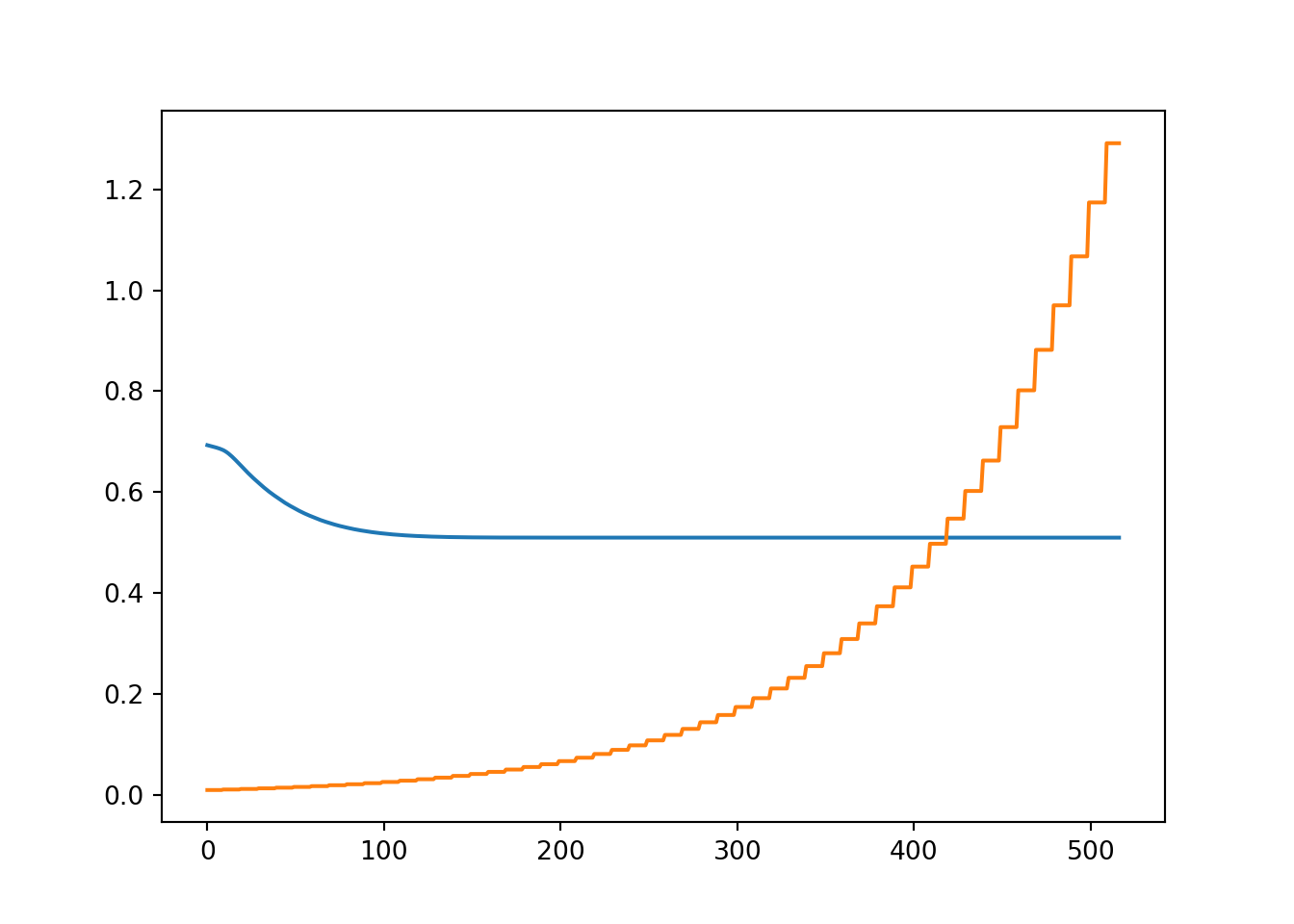

Testing the model

First, a quick wrapper function that returns a binary array of predictions: 0 = not a one-room floor plan; 1 = one-room floor plan.

def predict(X, params):
    yhat, steps = forward(X, params)
    return (yhat > .5).astype(int)

Next, we need to use the previously learnt parameters stored in m1 and pass the test dataset to predict().

pred = predict(X_test, m1["params"])

Finally, let’s calculate the classification accuracy:

acc_test = float((np.dot(Y_test.T, pred) + np.dot(1 - Y_test.T, 1 - pred)) / float(Y_test.size) * 100)

Our simple model correctly classified 79.3% of the floor plans in the training set and 80.1% of the floor plans in the test set.

Not amazing but given that the model only uses raw pixel values of the images, it’s not that bad either.

Footnotes

1. I am really not sure if the terminology and notation are technically correct. The equations below represent the individual steps for the back propagation simultaneously over all examples. The outputs of the individual steps range from scalar to matrix. Whether or not “derivative” is the appropriate term, I don’t know. I’m just a dumdum ¯\_(ツ)_/¯